Research
, Volume: 0( 0)Interpreting the UniverseâÂÂs Expansion Redshift Data with Respect to Energy
- *Correspondence:
- Benjamin T Soloman , Chairman, Xodus One Foundation, 4033 Palmwood Dr #8, Los Angeles, CA 90008, USA, Tel: 310-666-3553; E-Mail: bts@XodusOneFoundation.org
Received: August 04, 2018; Accepted: September 14, 2018; Published: September 19, 2018
Citation: Solomon BT, Beckwith AW. Interpreting the Universe?s Expansion Redshift Data with Respect to Energy. J Space Explor. 2018;7(3):148
Abstract
This paper extends the Law of Consistency to include transfer, transformation, keno and spectrum consistencies. Consistency at any scale therefore falsifies any theoretical approach that breaks the conservation of mass-energy. With these it is now possible to structure the expansion redshift data and propose how to handle uncertainties in the gravitational red shifts. A review of some of the latest finding point to precision in modern methods for estimating the expansion redshift, however, significant variable bias is present and therefore, accuracy eludes us. Proposing the shape of the Universe as the surface of a sphere, it was possible to identify sources of the heteroscedastic errors. These errors are primarily due to combining age with distance. Hubble Constant is found to be 75.403.
Keywords
Hubble; energy conservation; expansion redshift; gravitational redshift; cephids
Introduction
An alternative to the contemporary definition of a velocity-variable Einstein Relativistic Spacetime (ERS) or K4, ERS (1) was proposed [1].
K4, ERS = {x,y,z,t)
That spacetime keno (derived from Greek for vacuum) K5 consists of a rich medium (2) that is different from dimensions and operates in the three-space, one-time and one-electric dimensions.
 (2)
(2)
This spacetime keno K5 is accompanied by the Lorentz-FitzGerald Transformation (LFT) and Newtonian Gravitational Transformation (NGT) that exists within this spacetime, for an environment e, and are expressed by their velocity-variable rulers (3),
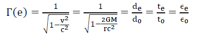 (3)
(3)
It was further proposed [1] that within spacetime, “the laws of physics are the same everywhere” can be crystallized, as the Law of Consistency, that the laws of the Universe are consistent everywhere and at every level of detail. There are two basic parts to this Law of Consistency.
The first, Transference Consistency (4), that any fundamental transformation present in spacetime Γs(x,y,z,t) must be identically mirrored on a particle Γp(x,y,z,t) in that local region and vice versa.
Γp(x,y,z,t) = Γs(x,y,z,t) Transference Consistency(4)
This is the reason why gravitational fields pass through all matter.
The second, Transformation Consistency (5), that all fundamental transformations are the same everywhere even though their origins are different. Or, given ρ, the general representation for a dimension’s ruler which is only a function of velocity and not the velocity gradient is,
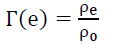 Transformation Consistency (5)
By the Transference Consistency (4) the modification of spacetime is evident as the energy of the particle. However, the spacetime distortion, though equivalent to energy, is not energy, else gravitational fields would deplete, but they don’t. Therefore, energy is an emergent property of spacetime.
The amount of modification present in spacetime can be measured by the energy of a particle. Transfer Consistency (4) goes both ways, from spacetime to particle, and from the particle to spacetime.
This raises two questions,
(i) If the deformed spacetime keno is not energy, then what is energy? And
(ii) What is this spacetime keno that alters our observations of dimensions? This paper focuses on the first question.
Motion requirement
The Law of Consistency, in particular, “at every level of detail”, requires that the energy within the transverse electromagnetic wave cannot oscillate between 0% and 100%. It must oscillate to and from somewhere. The solution proposed [2,3] was that the electromagnetic wave’s electric and magnetic vectors rotate between spacetime K5 and subspace K3 (x,y,z) and their projections on spacetime keno K5 are observed as transverse waves. There are two consequences:
(i) This expands the scope of Transference Consistency (4) to between kenos (6) or Keno Consistency,
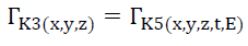 Keno Consistency (6)
(ii) Photon energy is the rotation of the electric and magnetic vectors between spacetime K5 and subspace K3 (x, y, z), but not due to these vectors’ field strength. This is confirmed by the fact that photon energy E (7) is purely a function of its frequency ν.
 (7)
(7)
As proposed [3-5] the maximum electric field strength EA is a function (8) of the photon’s wavelength λP and electric permittivity ε,
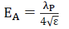 (8)
(8)
Therefore, one infers that for energy to manifest, the motion is a requirement.
Local distance phenomenon
A Ni field is a spatial gradient of real or latent velocities that are orthogonal to the direction of the acceleration. This acceleration, governed by (9), is in the direction of increasing orthogonal velocities. Gravity is a Ni field as one observes that a satellite’s orbital velocity increases as the radius of the satellite’s orbit decreases, and the gravitational acceleration increases as this radius decreases. Within spacetime Ni field forces [6-8] are governed by the massless formula for gravitational acceleration (9) and is valid for mechanical and electromagnetic forces.
 (9)
(9)
where τ is the spatial gradient of the time dilation transformation or change in time dilation transformation, divided by the distance r of this change. Noting that the time dilation transformation is the ratio of tv/t0 per LFT and NGT. That is, (9) is the universal mathematical descriptor of acceleration for macro forces.
Denoting δE the change in energy, δT the change in this time dilation transformation tv1/t0 to tv2/t0 across a distance δr from r1 to r2 that results in a change in velocity of a particle of mass m, from v1 to v2, from (9) gives,
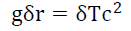 (10)
(10)
By the classical velocity-acceleration-distance equation,
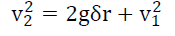 (11)
(11)
Or
 (12)
(12)
From (10) and (12),
 (13)
(13)
That is, by (9) and (10), spatial displacement is a necessary requirement for a particle to gain or lose energy. The particle’s energy gain/loss (13) in a deformed keno is a local phenomenon that is only dependent on the mass-energy of the particle. By mathematical induction, one can prove that this energy gain or loss is the same as the particle energies. Substituting for E=mc2 gives
 (14)
(14)
Noting (5) that transformations present are independent of their origins, a particle’s energy, and thus its structure, is enclosed by its own local set of transformations governed by the particle structure keno Kp and obeys Keno Consistency (6). It was proposed that this particle keno is the Variable Electric Permittivity (VEP) matter evidenced as binding energy, but much work remains [3].
Therefore, one infers that for energy to manifest, spatial displacement is a requirement.
Local probabilistic phenomenon
Using the Probabilistic Wave Function [2-5,8], an alternative to the Schrödinger Wave Function, it was shown [5] that the 1-dimensional deformation of subspace (15) along the orthogonal radius rP of the photon motion, determined by this photon energy is given by (16),
 (15)
(15)
 (16)
(16)
That is, Transformation Consistency exists in the subspace keno K3,SS. In the presence of non-linear transformations, such as NGT, the probabilistic deformation with respect to increasing photon energy is given by (17)
 (17)
(17)
where PN is the non-modulated (by the wave function) photon probability at a distance rP from the z-axis of photon propagation. Like NGT in spacetime, there exists an equivalent non-linear transformation in subspace. That is, it is possible to modulate probabilistic density in subspace, the equivalent of acceleration in spacetime.
The common denominator, energy, has different effects on different kenos depending on the properties of the keno. In spacetime, motion displacement is governed by velocity and acceleration, and in subspace, translocation is governed by probability and density, respectively.
That is, there are two known types of physical displacement, motion displacement, and translocation. Both are governed by vectoring (velocity and probability) and modulation (acceleration and density).
Energy is the change in physical displacement and is time invariant. This is observable in gravitational fields. The energy gained by a particle from velocity v1 to v2 is independent of the gravitational field strength and not dependent upon how slowly or quickly this energy is gained. Power, on the other hand, is determined by the strength of the gravitational field in that local region, and greater the strength the quicker the gain in this energy.
Structuring the expansion redshift data
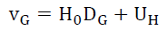
In this section, the authors will scrub and structure the empirical Hubble Law (18) data to determine what useful information there is to explain the differences in the observed Hubble constant H0 which ranges between 67.6 and 76.9 given galactic velocity vG and galaxy distance DG.
 (18)
(18)
One can model the uncertainty UH in the empirical Hubble Law data as follows,
 (19)
(19)
Where the uncertainties in the gravitational red shifts are, (i) UG introduced by the galaxy’s mass, rotation, and plane of rotation, (ii) US introduced by the identifying the star and its mass that created the photon per [1,3] the isotopic gravitational constant Gi, (iii) UI introduced by the spherical property [1] of the originating star that causes an additional redshift as the photon travels from inside the star to its surface, (iv) UT introduced by the technology used to determine the value of the Hubble’s constant, and (v) UE introduced by the unknown factors and alters the specific value of galactic velocity in that local region. Rewriting (18) gives
 (20)
(20)
It was proposed [1] that the Universe had to be a closed system, and therefore the total mass-energy is constant throughout the existence of the Universe. An explosion analog of the Universe implies a decelerating expansion if older and nearer galactic velocity vG is less than younger and further galactic velocity vG, while an accelerating expansion reverses this chronology [9,10]. The data shows something different and hidden factors may be present. Therefore, setting aside contemporary theories about galactic expansion, is it possible to structure this data to determine a good empirical model?
See TABLE 1 [11-32] for the data used to determine a structure.
| Index | Date published | Hubble constant | Error Range | Distance, D | Observer | Citation |
|---|---|---|---|---|---|---|
| (km/s)/Mpc | Mpc | |||||
| 1 | May-16 | 73.24 | ±1.74 | 30 | Hubble Space Telescope | [11] |
| 2 | May-01 | 72 | ±8 | 30 | Hubble Space Telescope Key Project | [12] |
| 3 | Apr-18 | 73.52 | ±1.62 | 30 | Hubble Space Telescope and Gaia | [13], [14] |
| 4 | Feb-18 | 73.45 | ±1.66 | 5 | Hubble Space Telescope | [15], [16] |
| 5 | Oct-17 | 70 | +12.0-8.0 | 41 | The LIGO Scientific Collaboration and The Virgo Collaboration | [17] |
| 6 | Feb-15 | 67.74 | ±0.46 | 4,139 | Planck Mission | [18], [19] |
| 7 | Jul-16 | 67.6 | +0.7-0.6 | 4,139 | SDSS-III Baryon Oscillation Spectroscopic Survey | [20] |
| 8 | Mar-13 | 67.8 | ±0.77 | 40 | Planck Mission | [21- 25] |
| 9 | Oct-13 | 74.4 | ±3.0 | Cosmicflows-2 | [26] | |
| 10 | Nov-16 | 71.9 | +2.4-3.0 | 2,612 | Hubble Space Telescope | [27] |
| 11 | Aug-06 | 76.9 | +10.7-8.7 | 3,985 | Chandra X-ray Observatory | [28] |
| 12 | Dec-12 | 69.32 | ±0.80 | 4,139 | WMAP (9-years), combined with other measurements. | [29] |
| 13 | Jul-05 | 70.4 | +1.3-1.4 | 4,139 | WMAP (7-years), combined with other measurements. | [30] |
| 14 | Jul-05 | 71 | ±2.5 | 4,139 | WMAP only (7-years). | [30] |
| 15 | Feb-09 | 70.5 | ±1.3 | 4,139 | WMAP (5-years), combined with other measurements. | [31] |
| 16 | Feb-09 | 71.9 | +2.6-2.7 | 4,139 | WMAP only (5-years) | [31] |
| 17 | Jun-05 | 70.4 | +1.5-1.6 | 4,139 | WMAP (3-years), combined with other measurements. | [32] |
Table 1: Hubble Constant, distance and source of data.
From this perspective, the WMAP data rows 12 to 17, can be eliminated as it produces many different values for H0 and therefore, the true value of H0 is masked by how the total error UH is processed. The data shows that many different methods were used and each arrived at a different number.
The Planck Mission (row 8) and Cosmicflow-2 (row 9) data were eliminated due to mix and large size reducing the possibility of determining distance measurements; that the errors introduced by UG, US, and UI, were not controlled for. Rows 10 to 11 were eliminated as these were large structures and suffers from all uncertainties UG, US, UI, and UE but UT. That leaves rows 1 to 7 for useful data.
Decelerating, static, or indeterminate universe
Using linear regression, the best model fitted (21) of the data gives a regression fit of 84.4%. See FIG. 1. This analysis suggests that Cepheids are good sources of Universe expansion estimates as these reduce the uncertainty UH due to the galactic mass, the spread of this mass, and the isotopic [1,3] gravitational constant at the time of the observation due to the local nucleosynthesis. That is, there is the need to more precisely determine what is happening rather than averaging a mass of data.

Figure 1: Hubble Constant versus Age in Mpc.
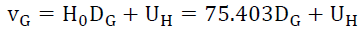
The regression equation (21), shows that the Hubble constant is a variable HD for a given star’s (age in) distance DG from an observer (in this case Earth), in the current time is,
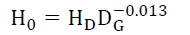 (21)
(21)
 (22)
(22)
Therefore, rewriting (20) gives (23),
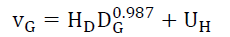 (23)
(23)
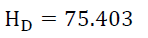
Equation 21 would explain why Hubble’s constant appears to be less the older the observed photon. However, an exponent of 0.987 does not make much sense. The most likely inference is that the exponent is 1 and that the errors in the data are heteroscedastic i.e. the error in the data is biased and these errors change with distance as evidenced by -0.013 exponents in (21). Hubble’s constant H0 is 75.403 or,
 (24)
(24)
With this value for Hubble’s constant one can recalculate Λ
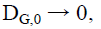
Using subscripts 0 and P (for past) to identify age of the Universe at the present and in the beginning respectively, as the stars and galaxies utilized to measure this expansion (relative to the observer) gets nearer or
 (25)
(25)
or, the expansion vG,P at the present time is no longer measurable, it is zero, and the uncertainty in the measurement becomes the dominant factor. That is nearby stars and galaxies are of immense value in determining the magnitude and sources of uncertainty. On the other hand, vG,0 the expansion at the beginning of the Universe,
DG,0 → 4,139 Mpc or 13.5 billion years ago,
 (26)
(26)
That is, spacetime as we know it formed under very energetic conditions, but that raises the question what was there before spacetime formed?
By Transfer Consistency (4) and Transformation Consistency (5), the observed original spectrum, now expansion redshifted, must be the same anywhere and anytime the photon was created (Spectrum Consistency), else this expansion redshift is noisy.
For example, it would be impossible to determine an isotope’s spectrum if the gravitational transformations did not change in a consistent manner across the isotope’s electron shell.
The empirical gravitational spectrum redshift vindicates this thesis. That is, Spectrum Consistency (27) requires that the photon’s spectrum at origination (from a transition structure St whether orbital, nuclei or particle) is independent of the environmental transformations (3) present to an observer in that same environment, given all other factors held the same. Or photon energy EP with frequency ν at origination, caused by a change in transition between states L1 and L2 is independent of the transformation, Γi present at the transition structure St.
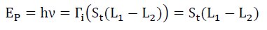 Spectrum Consistency (27)
So, is the Universe expanding? There are three possible theses:
a. Decelerating: Expansion is decelerating as nearer at 30 Mpc, older, galactic velocity vG is 2,262 km/s and further at 4,139 Mpc, younger galactic velocity vG is 312,093 km/s. See FIG. 2. This expansion redshift shows that the Universe appears to be cooling or decelerating.
b. Static: (23) and (24) informs that the Universe cannot be expanding in the current time, but the expansion shows that redshift is present i.e photons lose energy as they traverse the Universe. Consider the gravitational analog. The closer a photon originates from the center of the gravitational field the more redshifted it is. Could the Universe be static, and mimic this gravitational analog in a consistent manner? Such a hypothesis would explain why this “expansion” is extreme in the early age.
c. Indeterminate: Expansion is relative to the observer, and therefore it is not possible, with the current data to determine exactly how the Universe is changing. This brings us back to the earlier question. What is the shape of the Universe? Noting its “isocentric” property that the Universe appears inside-out and the observer is always at the center of the observer’s Universe.
That the beginning of the Universe, it’s youngest most distant part with the greatest relative expansion redshift, is observable furthest away from us in every direction one looks. It’s the oldest and nearest part, our current time with zero relative expansion redshift is a point closest to the observer FIG. 2.

Figure 2: Expansion Velocity (km/s) versus Distance (Mpc).
Any hypothesis about a changing Universe, needs to propose a shape of the Universe that explains this isocentric property, that
(a) The apparent inside-out structure of the Universe
(b) The relative redshift with respect to the age of the star or galaxy, and
(c) The zero, relative expansion of the Universe in our current time.
As Einstein had suggested many decades ago (reference lost) the Universe as a surface of a sphere would satisfy (a) and (b). It could possibly (c) if the Universe is large enough.
Shape and constraints
Assuming that, the expansion redshift is aligned with the gravitational redshift, by the Law of Consistency, the Static Hypothesis implies that the expansion redshift adds to the gravitational redshift and therefore adds to the gravitational escape velocity. Calculating the equivalent GM (per [1,3] the gravitational constant is a variable determined by the isotopic mass of the element) FIG. 3 shows the variation of the empirical GM across the age of the Universe. It is a function (28) of distance (current interpretation of age) of the Universe.

Figure 3: Empirical GM versus Distance (Mpc).
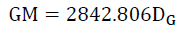 (28)
(28)
Consider that the gravitational coefficient was necessarily different in the past GP and from what it is now G0 due to nucleosynthesis and the arrangement of matter [1,3]. (28) can be rewritten as (29) and (30),
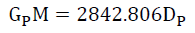 (29)
(29)
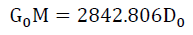 (30)
(30)
Or
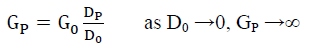 (31)
(31)
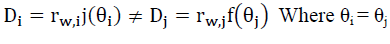
That is, using the Universe’s relative expansion, the beginning conditions are indeterminate. The physical reason for this is straightforward. The Universe is the surface of a sphere in some w dimensions, and the redshifted age is the arc distance Di (32) where i ranges between 0 and P, on this surface, and not the radius rw,i of this sphere. Assuming that, there exists a set of w dimensions (wx,wy,wz) corresponding to the (x,y,z) dimensions.
 (32)
(32)
where θi is the arc angle from the true center of Universe
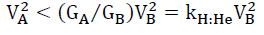
It is now possible to reduce the noise UH in the data, by inferring some boundary conditions:
For observable photons, the relative expansion velocity vG cannot be greater than the velocity of light c.
 (33)
(33)
Surface relative expansion necessarily implies a radial expansion rw,j (younger further away galaxies) to rw,i (older nearer galaxies) is governed by,
 (34)
(34)
 (35)
(35)
That is, for two photons i and j coming from the same arc angle θi = θj must originate from different radii ww,i and rw,j such that photon j is differently relative expansion redshifted (24) than ‘i’ see FIG. 4, For example, the expansion redshift of galaxy j is greater than that of the galaxy because it is closer to the origin of the Universe. However, the photons’ path distances measured are different.

Figure 4: Universe as the surface of a sphere at time i and j, with same arc angle.
 (36)
(36)
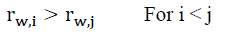
That is, for two photons i and j coming for the same radius rw,i ≠ rw,j must originate from same arc angles θi and θj such that photon j is differently relative expansion redshifted (24) than ‘i’ see FIG. 5. For example, the expansion redshift of galaxy ‘j’ is greater than that of the galaxy ‘i’ because it is closer to the origin of the Universe. However, the photons’ path distances measured are the same.

Figure 5: Universe as the surface of a sphere at time i and j, with same arc angle.
Therefore, it is clear there are several sources of errors.
The shape of the universe: The redshift observations are determined by the arc path of the Universe from a smaller radius rw,j to a larger radius rw,i. If this thesis, the Universe is the surface of a sphere in the w dimensions, is correct, then the expansion observations are composed of many different radii of the Universe. This is different from current theoretical models that assume just 4-dimensional spacetime.
Measurement methodology: FIG. 4 and 5 shows that distance is the length of the path taken by the photon which is best measured by a parallax method. That the two factors present are the Universe expansion redshift due to distance and Universe age redshift due to radii.
Mirages: Much of what is observed are mirages, that galaxies are close together but have no observable gravitational interaction. FIG. 4 and 5 illustrate how a photon’s path to an observer can originate from many different “locations”, along with any radius from a past Universe structure. [9] provides a good survey of anomalous expansion redshift data, stating “Measurements of the macro universe are odd, revealing exceptions more than the rule”.
Combined factors: Heteroscedastic errors in the redshift data are due to interpreting two factors, spacetime distance and Universe structure radii, as a single factor, age-distance. These are errors in the data due to combined age (radii) and spacetime distance and can only be addressed by separating out these two factors.
Accuracy versus precision
Let us step back a little. There are three important concepts in statistics, precision or spread, accuracy, and bias. Precision refers to the closeness of two or more measurements to each other. The variations in the measurements are due to random errors. Accuracy refers to the closeness of a measured value to a known true value. That is, a true value must be known. Bias is the tendency of a measurement to deviate in a repeatable manner from the true value due to systematic errors. Therefore, in the absence of a known true value, it is impossible to determine the bias in the measurements.
From the perspective of precision, the LIGO Scientific Collaboration and The Virgo Collaboration [10], sums it elegantly, “A plethora of methods exist to estimate H0, using Cepheid variables, red-giant stars, SNe, gravitational lenses, galaxies, the CMB and neutron-star mergers. The best cosmology-independent constraints come from the SH0ES Cepheid-SN distance ladder; the tightest constraints come from the Planck CMB data, assuming a standard ΛCDM cosmology.
These estimates are discrepant at the 3-σ level, corresponding to odds of 10:1 of ΛCDM being the correct model. Numerous attempts have been made to reconcile the two results through new physics or improved astrophysical, experimental and statistical modeling, yielding no compelling explanation. Here, we look to the inverse distance ladder and Gravitational Wave (GW) standard sirens to provide the independent information needed to arbitrate this tension, which we frame in a new, intuitive way using the Posterior Predictive Distribution (PPD)”.
That is, a very substantial amount of sophisticated analysis had been applied to improve the precision with the implicit assumption that this would lead to improved accuracy. However, in the absence of a known true value, it is not possible to determine the bias in these measurements. The 3-σ discrepancy strongly suggests that bias is present. The errors being heteroscedastic point to a bias that varies with undetermined factors.
The isotopic [1,3] gravitational coefficient ‘Gi’ thesis would imply (i) Only methods that are based on motion mechanics could provide good estimates of the total redshift, however noting that redshift analysis is now a three-variable (gravitational acceleration ‘g’, gravitational mass ‘M’, and the composite gravitational coefficient problem ‘Gi’) and not two-variable (‘g’ and ‘M’) problem requires additional attention to detail to determine these parameters.
Clearly, other non-motion mechanics-based methods on the distance ladder would have to be recalibrate if the isotopic gravitational coefficient thesis is correct.
This implies that the neutron star’s photon gravitational redshift would be less than currently estimated using GE. The Universe expansion redshift would contribute a larger component to the total observed redshift, that is, neutron stars are further away than they appear to be. The lower [10] Hubble constant H0 of 70 and would be consistent with (23) given the H0 range of +12.0 and −8.0.
And (ii) ΛCDM is dependent on the constancy of the gravitational constant GE. Given an isotopic gravitational coefficient Gi thesis, in the presence of nucleosynthesis, this constancy would no longer hold.
Therefore, the isotopic gravitational coefficient Gi thesis illuminates two biases
(i) Biases at photon origination from the observed star, and
(ii) Biases at detection through the use of theoretical models that require a time-invariant gravitational constant GE. This justifies eliminating data between rows 8 to 17 of TABLE 1.
An alternative to the dark matter thesis
If the mass M of the Universe is constant across its age, then the gravitational constant G increases with distance back into the past or decreases with increasing age of the Universe. The isotopic [1,3] gravitational coefficient Gi could be consistent with (28). The missing mass of the Universe, as measured by GM and assuming G is a constant across age, would account for a substantial proportion of the missing mass, if at all. From [1,3] the gravitational coefficient G determined by the aggregation constant ka,R and the isotopic constant kiso per (37),
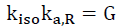 (37)
(37)
where ka,R = 2.24417070379951x10+25, kiso is given by (38), for isotope ‘i’ with mass ‘Mi’,
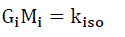 (38)
(38)
Therefore, (28) can be rewritten in terms of the number of particles n as,
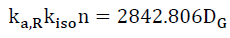 (39)
(39)
The proper method to solving (39) is to document each star, its composition, mass, redshifts, etc. and use a search algorithm to minimize the errors. There are two quick and dirty approaches to solving (39). First, assuming that n is essentially a constant, as mass is essentially constant, find the ratios of aggregation constant ka,R for the various observations ‘i’ and ‘j’ from 1 to 7 of TABLE 1, such that,
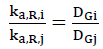 (40)
(40)
For the data, this ratio ranges between 6 and 138 and suggests that significant changes in the aggregation of matter, from the early Universe to the present day is partially responsible for the changes in the Universe’s expansion redshift. This is the same conclusion from the analysis of the anomalous galaxy rotations.
With regard to these anomalous galaxy rotations, it was shown [1,3] that for outward expansion, a star’s rotational radius RB with rotational velocity VB, before 1H:4He nucleosynthesis and rotational radius RA with rotational velocity VA after 1H:4He nucleosynthesis is given by,
 (41)
(41)
 (42)
(42)
Where GB and GA are the composite gravitational coefficients before and after the 1H:4He conversion, respectively. By conservation of energy, for a star of mass m, and central galactic mass M, the total kinetic and potential energy, before TB and after TA must be the same,
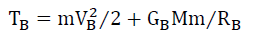 (43)
(43)
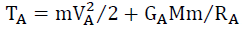 (44)
(44)
And it was shown that,
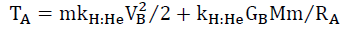 (45)
(45)
Therefore,
 (46)
(46)
And by Conservation of Mass and Energy, there is a missing energy component f(GA) which is currently proposed as the dark matter thesis.
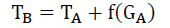 (47)
(47)
As required by Transference Consistency (4) the modification of spacetime is evident as the energy of the particle. However, the spacetime distortion, though equivalent to energy, is not energy, and therefore, one observes apparent deviations from conservation of mass-energy.
Conclusion
The Law of Consistency consists of 4 parts, (i) Transferences, (ii) Transformation, (iii) Keno, and (iv) Spectrum Consistencies. Associated with this are the two requirements for energy to manifest at a particle level are, (a) motion, and (b) spatial displacement, at every level of detail. That is, the Universe is rigorously consistent at every level of detail whether at the particle level or the galactic level.
Consistency at any scale, therefore, falsifies any theoretical approach that breaks the conservation of mass-energy. As a result, using the isotopic gravitational coefficient thesis, this paper has taken a step towards proposing a shape for the Universe that could explain observed gravitational anomalies and account for biases in the measurements.
References
- Solomon BT, Beckwith AW. Exploring the Foundations of Gravity Using Empirical Data. J Space Explor. 2018;7.
- Solomon BT, Beckwith AW. Probability, Randomness & Subspace, with Experiments. J Space Explor. 2017;6.
- Solomon BT. Unifying Gravity with the Atomic Scale, Scholar?s Press, 2017
- Solomon BT. Beckwith AW, Photon Probability Control with Experiments. J Space Explor. 2017;6.
- Solomon BT. Beckwith AW, Probability as a Field Theory. J Space Explor. 2017;6.
- Solomon BT. An Introduction to Gravity Modification, Universal Publishers, Boca Raton, 2nd Edition 2012.
- Solomon BT. Gravitational Acceleration without Mass And Non-inertia Fields, Physics Essays, 2011;24:327.
- Solomon BT, Beckwith AW. Probabilistic Deformation in a Gravitational Field. J Space Explor. 2017;6.
- Ratcliffe H. A Review of Anomalous Redshift Data, 2nd Crisis in Cosmology Conference, CCC-2 ASP Conference Series. 2009;413.
- Feeney, Stephen M, Peiri et al. Prospects for resolving the Hubble constant tension with standard sirens. 2018.
- Riess AG, Macri LM, Hoffmann SL, et al. A 2.4% Determination of the Local Value of the Hubble Constant. Astrophys J. 2016;826:56.
- Freedman WL. Final results from the Hubble Space Telescope Key Project to measure the Hubble constant. Astrophys J. 2001;553:47-72.
- Riess AG, Casertano, Stefano, et al. Milky way cepheid standards for measuring cosmic distances and application to gaia dr2: implications for the hubble constant. 2018.
- Devlin, Hannah. The answer to life, the universe and everything might be 73 or 67. The guardian. 2018.
- Riess AG, Casertano, Stefano et al. New parallaxes of galactic Cepheids from spatially scanning the Hubble Space Telescope: Implications for the Hubble constant . Astrophys J. 2018.
- Weaver D; Villard R, Hille K. Improved hubble yardstick gives fresh evidence for new physics in the universe. NASA. 2018.
- The LIGO Scientific Collaboration and The Virgo Collaboration; The 1M2H Collaboration; The Dark Energy Camera GW-EM Collaboration and the DES Collaboration; The DLT40 Collaboration; The Las Cumbres Observatory Collaboration; The VINROUGE Collaboration; The MASTER Collaboration . A gravitational-wave standard siren measurement of the Hubble constant. Nature. 2017.
- Planck Publications: Planck 2015 Results. European Space Agency. 2015.
- Cowen R, Castelvecchi D. European probe shoots down dark-matter claims. Nature. 2014.
- Grieb JN, Sánchez AG, Salazar AS. The clustering of galaxies in the completed SDSS-III Baryon Oscillation Spectroscopic Survey: Cosmological implications of the Fourier space wedges of the final sample. Monthly Notices of the Royal Astronomical Society. 2016
- Bucher PAR. Overview of products and scientific Results. Astron & Astrophys. 2013;571:A1.
- Planck reveals an almost perfect universe. ESA. 2013.
- Planck Mission Brings Universe Into Sharp Focus. JPL. 2013.
- Overbye D. An infant universe, born before we knew. New York Times. 2013.
- Boyle A. Planck probe's cosmic 'baby picture' revises universe's vital statistics. NBC News. 2013
- Tully RB, Courtois HM, Dolphin AE, et al. Cosmicflows-2: The Data. Astron J. 2013;146:86.
- Bonvin V, Courbin F, Suyu SH, et al. H0LiCOW-V. New COSMOGRAIL time delays of HE 0435-1223: H0 to 3.8 per cent precision from strong lensing in a flat ?CDM model. MNRAS. 2016;465:4914-30.
- Bonamente M, Joy MK, Laroque SJ, et al. Determination of the cosmic distance scale from Sunyaev?Zel'dovich effect and Chandra X-ray measurements of high-redshift galaxy clusters. Astrophys J. 2006;647:25.
- Bennett CL. Nine-year Wilkinson Microwave Anisotropy Probe (WMAP) observations: Final maps and results. Astrophys J Supplement Series. 2013;208:20.
- Jarosik N. Seven-year Wilkinson Microwave Anisotropy Probe (WMAP) observations: Sky maps, systematic errors, and basic results. Astrophys J Supplement Series. 2011;192:14.
- Hinshaw G. Five-year wilkinson microwave anisotropy probe observations: data processing, sky maps, and basic results. Astrophys J Supplement. 2009;180:225-45.
- Spergel DN. Three-year wilkinson microwave anisotropy probe (wmap) observations: Implications for cosmology. Astrophys J Supplement Series. 2007;170:377-408.